Na-enyocha ọtụtụ PivotTables n'otu oge

When creating complex reports and, especially, dashboards in Microsoft Excel, it is very often necessary to simultaneously filter several pivot tables at once. Let’s see how this can be implemented.

Method 1: General Slicer for filtering pivots on the same data source

If the pivots are built on the basis of one source data table, then the easiest way is to use them to filter them simultaneously ngalaba is a graphic button filter connected to all pivot tables at once.

To add it, select any cell in one of the summary and on the tab analysis họrọ otu Tapawa Mpekere (Analyze — Insert slicer). In the window that opens, check the boxes for the columns by which you want to filter data and click OK:

The created slicer will, by default, filter only the pivot for which it was created. However, using the button Report Connections (Report connections) tab iberi (Slices) we can easily add other summary tables to the list of filtered tables:

Method 2. General slice for filtering summaries on different sources

If your pivots were built not according to one, but according to different source data tables, then the above method will not work, because in the window Report Connections only those summaries that were built from the same source are displayed.

However, you can easily get around this limitation if you use the Data Model (we discussed it in detail in this article). If we load our tables into the Model and link them there, then the filtering will apply to both tables at the same time.

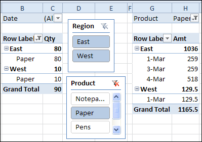
Let’s say that we have two tables for sales and transportation costs as input data:

Suppose that we are faced with the task of building our own summary for each of them and then filtering them simultaneously by cities with a common cut.

Anyị na-eme ihe ndị a:

1. Turning Our Original Tables into Dynamic Smart Tables with a Keyboard Shortcut Ctrl+T ma ọ bụ iwu Ụlọ - Ụdị dị ka tebụl (Ụlọ - Ụdị dị ka tebụl) and give them names tablProdaji и tabTransport tab Onye isi ike (Kere).

2. Load both tables in turn into the Model using the button Tinye na ụdị data on the Power Pivot tab.

It will not be possible to directly link these tables in the Model, because while Power Pivot only supports one-to-many relationships, i.e. requires one of the tables to have no duplicates in the column we are linking on. We have the same in both tables in the field mmetụta there are repetitions. So we need to create another intermediate lookup table with a list of unique city names from both tables. The easiest way to do this is with the Power Query add-in functionality, which has been built into Excel since the 2016 version (and for Excel 2010-2013 it is downloaded for free from the Microsoft website).

3. Having selected any cell inside the “smart” table, we load them one by one in Power Query with the button Site na tebụl / nso tab data (Data - Site na tebụl / nso) and then in the Power Query window select on isi ìgwè Close and load – Close and load in (Ụlọ - Mechie&Buchie - Mechie&Buchie na…) and import option Naanị mepụta njikọ (Naanị mepụta njikọ):

4. We join both tables into one with the command Data – Combine Queries – Add (Data — Combine queries — Append). Columns with the same names in the header will fit under each other (like a column mmetụta), and those that do not match will be placed in different columns (but this is not important for us).

5. Delete all columns except column mmetụtasite na ịpị aka nri na aha ya wee họrọ iwu Hichapụ ogidi ndị ọzọ (Wepu ogidi ndị ọzọ) and then remove all duplicate city names by right-clicking the column heading again and selecting the command Wepu oyiri (Remove duplicates):

6. The created reference list is uploaded to the Data Model via Ụlọ - Mechie na ibu - Mechie ma buo ya (Ụlọ - Mechie&Buchie - Mechie&Buchie na…) ma họrọ nhọrọ Naanị mepụta njikọ (Naanị mepụta njikọ) and the most important thing! – turn on the checkbox Tinye data a na ụdị data (Tinye data a na ụdị data):

7. Now we can, returning to the Power Pivot window (tab ike pivot - bọtịnụ Management), switch to Nlele eserese (Diagram view) and link our tables of sales and transportation costs through the created intermediate directory of cities (by dragging fields between tables):

8. Now you can create all the required pivot tables for the created model using the button tebụl nchịkọta (Pivot Tebụl) on isi (Ulo) tab in the Power Pivot window and, by selecting any cell in any pivot, on the tab analysis add slice button Tapawa Mpekere (Analyze — Insert Slicer) and choose to slice in the list box mmetụta in the added directory:

Now, by clicking on the familiar button Report Connections on Slice tab (Slicer — Report connections) we will see all our summary, because they are now built on related source tables. It remains to enable the missing checkboxes and click on OK – and our slicer will start filtering all selected pivot tables at the same time.